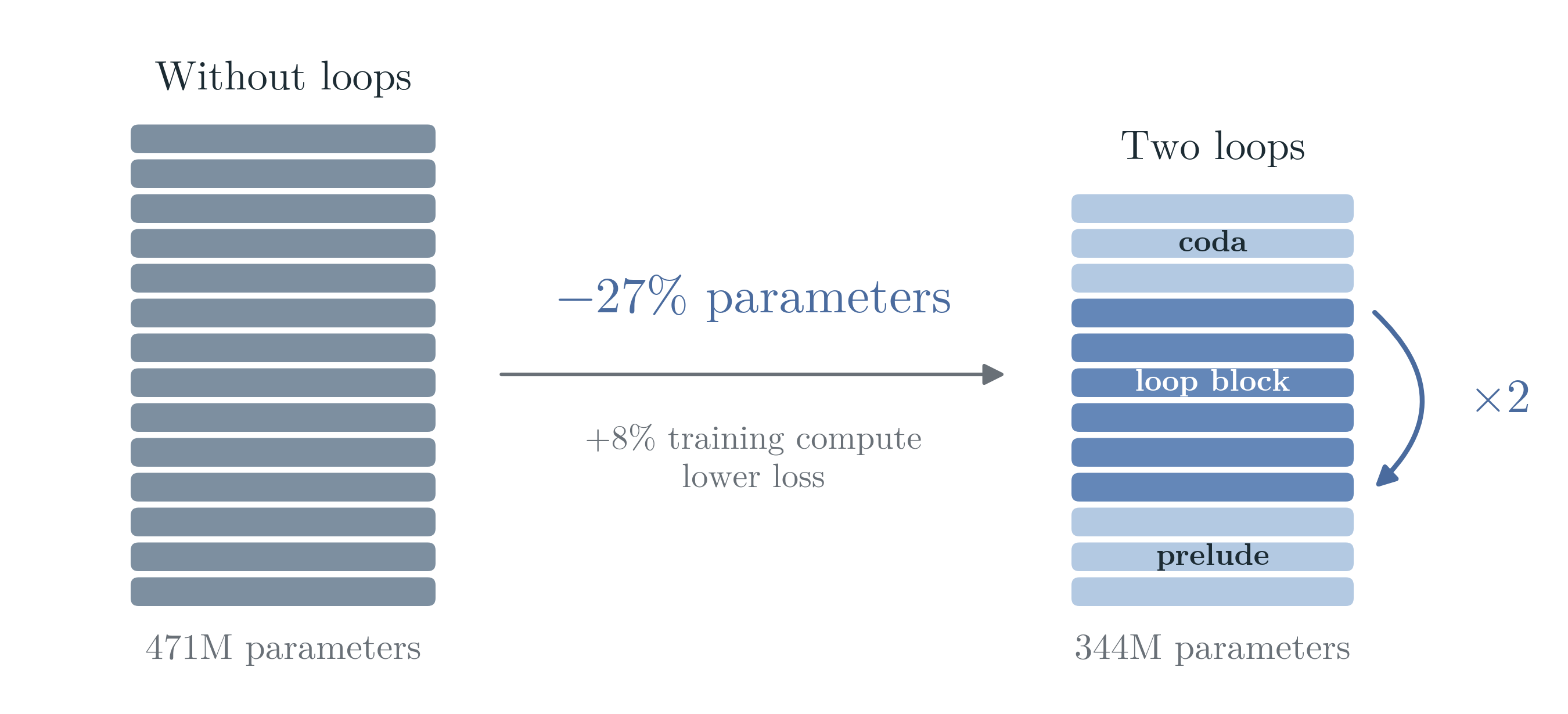
The Benefit of Looping Twice:Parameter Savings with Little Added Compute
Looped transformers at matched training compute, in dense models and in mixture-of-experts
Cite this work
@article{xiong2026truncate,
  title   = {Truncate or Not? A Scaling Study of Looped Transformers
             with Truncated Backpropagation},
  author  = {Xiong, Xuyuan and Chen, Siyu and Shao, Zihan and Su, Yue
             and Jin, Weiyang and Luo, Ping and Yang, Zhuoran and Liu, Xihui},
  journal = {arXiv preprint arXiv:2610.26030},
  year    = {2026}
}
TL;DR
A looped transformer reuses one block of layers several times for every token. We ask how many parameters this saves against a standard transformer trained with the same compute, measure it in dense and in mixture-of-experts models, and explain it with a scaling law fitted to nearly 600 training runs.
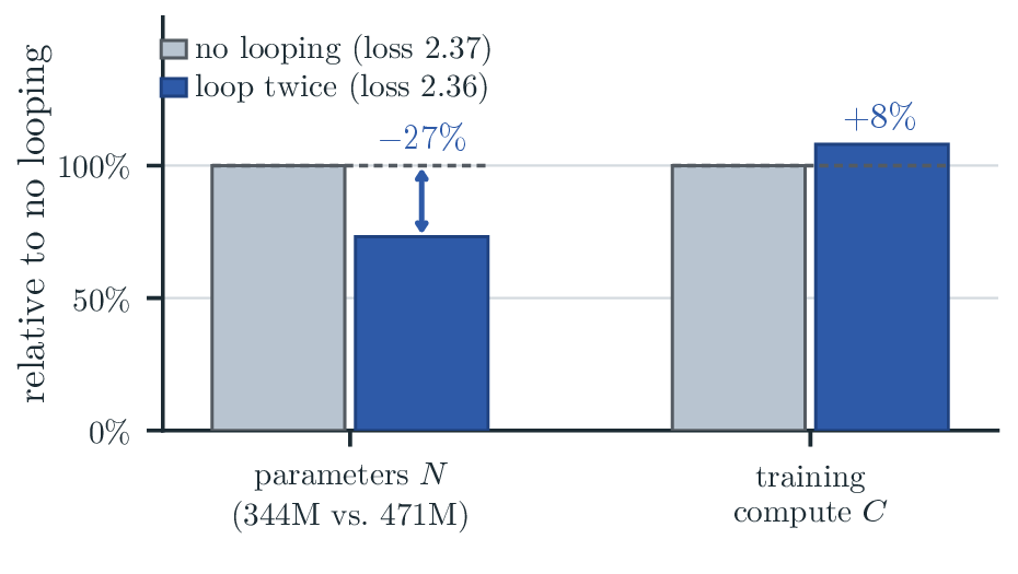
- Dense models. With 27% fewer parameters, a 344M looped model reaches a lower loss than the best 471M model without loops, for 8% more training compute.
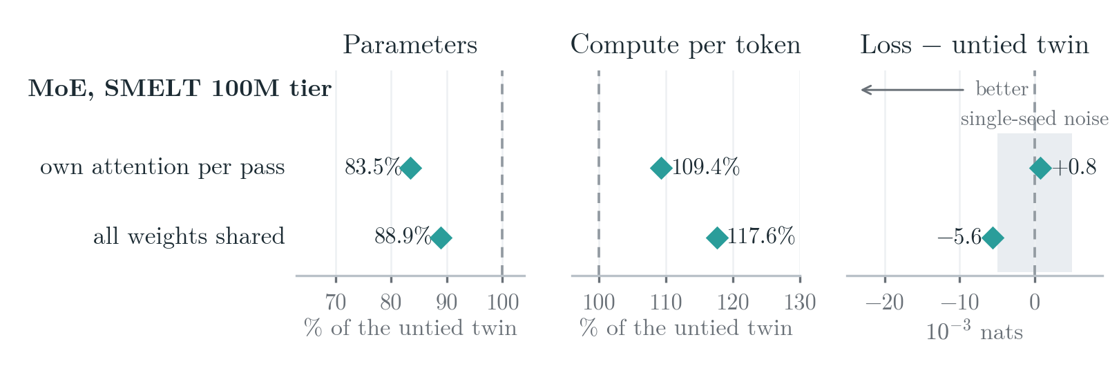
- Mixture-of-experts. A looped model that shares its experts across its two passes matches its untied counterpart with 17% fewer parameters and 9% more compute per token; a purely looped model beats it with 11% fewer parameters and 18% more compute per token.
- Why two loops. A scaling law prices a loop in effective parameters. Read at equal loss, it gives a Pareto frontier of parameters saved against compute paid. Two fully trained loops are its knee: they give most of the attainable parameter saving for a few percent more compute.
| Looped model | Parameters saved | Extra compute | Loss vs reference |
|---|---|---|---|
| Against the best model without loops | |||
| Dense (2, 2), same compute | 27–32% | 0% | +0.001 to +0.008 |
| Dense (2, 2), 8% more tokens | 27% | +8% | −0.007 |
| Against the untied model, on the same tokens | |||
| Dense (2, 2), widened | 19–21% | +15–22% | −0.005 to −0.017 |
| MoE, own attention per pass | 17% | +9% | +0.001 |
1. Introduction
Looped transformers apply one block of layers several times for every token, so they add depth without adding weights. This is usually read as more computation for the same parameters. We read it the other way round. Parameters are what a model costs to store, move and serve, and training compute is what it costs to make; the two budgets are often separate, since a model trained once on a cluster may later run on hardware with a fixed amount of memory. At the same training compute and the same loss, how many fewer parameters does a looped model need?
Recent work on looped mixture-of-experts models, SMELT [1], matches a looped model to its baseline in parameters, per-token compute and KV cache, and finds that looping still lowers the loss: on the compute-optimal frontier it saves 6.8–18% of the training compute. We ask a different question: when the parameter count is free to fall, how many fewer parameters does a looped model need for the same loss, and how much extra compute does that cost? It is the question behind the free-size results of our paper, Truncate or Not? A Scaling Study of Looped Transformers with Truncated Backpropagation [2].
The rest of this post follows three questions.
- First, does a loop save parameters in practice? It does. A dense looped model with 27% fewer parameters beats the best model without loops for 8% more training compute (Section 3).
- Second, does the saving carry over to mixture-of-experts models? It does. Sharing the experts across two passes saves 17% of the parameters at matched loss for 9% more compute per token, and a purely looped model beats its untied twin with 11% fewer parameters and 18% more compute per token (Section 4).
- Third, why two loops? A scaling law fitted to nearly 600 training runs prices a loop in effective parameters: two fully trained loops are worth 1.91 copies of the looped block. Read at equal loss, the law gives a parameter–compute Pareto frontier whose knee is two fully trained loops, saving about a third of the parameters for 3% more compute (Sections 5 and 6).
2. Looped Models
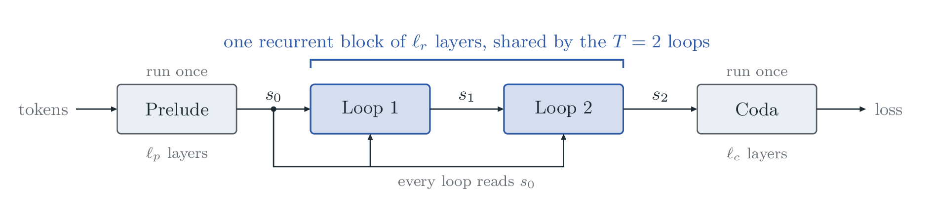
We use the prelude–recurrent–coda architecture of Geiping et al. [3] and Schwethelm et al. [4]. A prelude maps tokens to hidden states, a shared recurrent block refines them over T loops, and a coda predicts the next token. A loop setting (T,B) runs T loops forward and backpropagates through the last B; B=T is full backpropagation through time (BPTT), and (1,1) is a standard transformer. The non-embedding parameters split into N=N_{\text{once}}+N_{\text{rec}}: the prelude and coda run once per token, the recurrent block runs in every loop (Fig. 1).
3. Parameter Savings in Dense Models
Finding 1: Two fully trained loops save 27–32% of the parameters at the same training compute. With 8% more training compute, a (2,2) model with 27% fewer parameters beats the best model without loops; against the untied model on the same tokens, looped models with a fifth fewer parameters win for 15–22% more compute per token.
We compare looped and standard dense models in two ways: compute-optimal pairs, and the untied model on the same tokens.
3.1 Compute-Optimal Pairs
At three training budgets, we train (1,1) and (2,2) each at the size and token count that minimize its own loss, with three seeds per model (Tab. 2).
| Compute (FLOPs) | (1, 1) size | (1, 1) loss | (2, 2) size | (2, 2) loss | Gap (10⁻³ nats) |
|---|---|---|---|---|---|
| 1.6 × 10¹⁸ | 115M | 2.7098 | 79M | 2.7177 | +7.9 ± 1.9 |
| 6.0 × 10¹⁸ | 239M | 2.5215 | 162M | 2.5253 | +3.8 ± 1.8 |
| 2.1 × 10¹⁹ | 471M | 2.3663 | 344M | 2.3677 | +1.4 ± 1.7 |
| 2.2 × 10¹⁹ (+8%) | 471M | 2.3663 | 344M | 2.3590 | −7.3 ± 1.8 |
At every budget the looped model has 27–32% fewer non-embedding parameters and nearly the same loss, and the gap closes as the budget grows, to 0.001 nats at 2.1\times10^{19} FLOPs. Trained on 8% more tokens, and so with 8% more compute, the 344M (2,2) model beats the 471M model without loops by 0.007 nats (Fig. 2).
3.2 Against the Untied Model
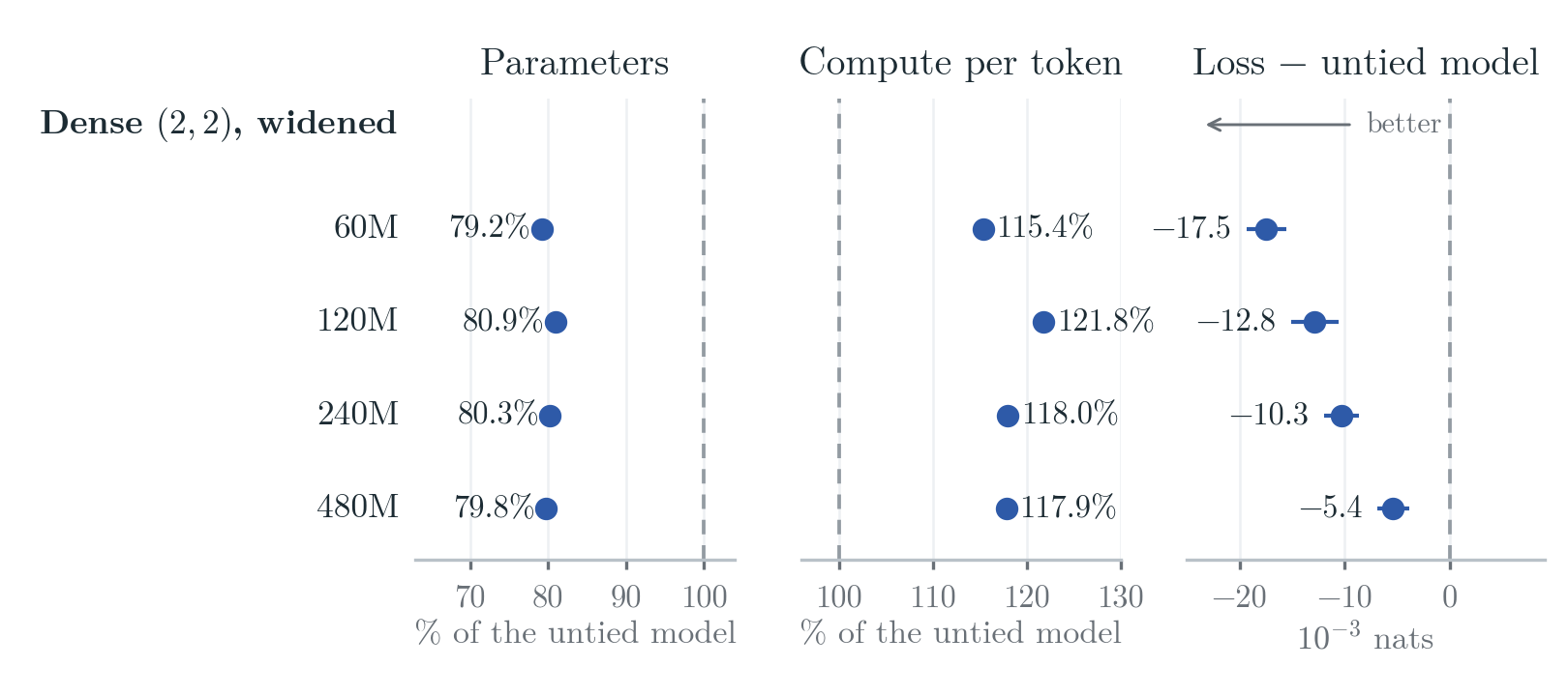
The pairs let both models choose their size. A tighter test keeps everything else equal: the untied model is the same network with a separate copy of the recurrent block for each loop. For two loops it has about 1.5 times the parameters at the same compute per token. We train both at four sizes on the same tokens, about 18 tokens per parameter of the looped model, with three seeds each.
At the untied model’s width the looped model trails it by 0.009–0.017 nats; widening it reverses the gap at every size (Fig. 3). Widened to about 80% of the untied model’s parameters, for 15–22% more compute per token, it beats the untied model by 0.005–0.017 nats in all twelve seed pairs.
4. Parameter Savings in Mixture-of-Experts Models
Finding 2: The saving carries over to mixture-of-experts models. A looped MoE model that shares its experts across its two passes matches its untied twin with 17% fewer parameters for 9% more compute per token; a purely looped one beats the twin with 11% fewer parameters for 18% more compute per token.
4.1 Configurations
The dense results show a trade: a loop saves parameters at the same loss for a little more compute. We test it in mixture-of-experts models, where the experts hold nearly all of the parameters, with the untied comparison of Section 3.2. The reference is the untied twin of SMELT’s 100M tier [1]: 10 layers of width 576 with 96 experts per layer (8 active per token), whose layers 3–7 run twice with separate weights for each pass, 1,068M non-embedding parameters in total. Both looped models have 11 layers and run their middle five twice; all three models train on the same 12.58B FineWeb-Edu tokens, with one seed each (Tab. 3).
- Shared experts. The first looped model, of width 592 with 104 experts per layer, shares the experts and the router between its two passes; they hold almost all of the parameters. Each pass keeps its own attention and norms, and the second pass’s copy adds only 0.5% to the parameter count. Foil [5] calls this untying the attention and finds that it lowers the loss of looped MoE models at no extra compute.
- Purely looped. The second shares every weight between its two passes. It is wider, with width 624 and 100 experts per layer.
| Model | Parameters | Compute per token | Loss − twin |
|---|---|---|---|
| Untied twin | 1,068M | 1.00 | — |
| Own attention per pass | 892M (0.835) | 1.094 | +0.0008 |
| All weights shared | 950M (0.889) | 1.176 | −0.0056 |
4.2 Results
Sharing the experts across the two passes saves 17% of the parameters at matched loss: the looped model with its own attention per pass matches the untied twin, at +0.0008 nats, for 9% more compute per token. The purely looped model, with 11% fewer parameters and 18% more compute per token, is 0.006 nats ahead. As in dense models, a looped model with fewer parameters than its untied twin matches or beats it for some extra compute per token (Fig. 4).
5. A Scaling Law for Looped Models
Why does looping twice save so much, and what do other loop settings save? A scaling law fitted to nearly 600 training runs answers both, by pricing every loop setting in effective parameters.
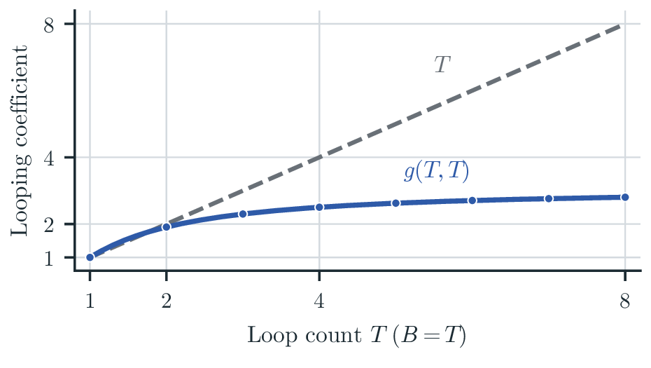
Finding 3: Two fully trained loops make the looped block worth 1.91 copies of itself. A loop setting (T,B) makes the block count g(T,B) times in an effective parameter count; fitted to nearly 600 training runs, g saturates at about three copies however often the block loops.
5.1 Effective Parameters
A loop can only enlarge the block that loops. We therefore write the loss with an effective parameter count N_{\text{eff}}, the size of a model without loops that reaches the same loss on the same tokens: the recurrent block counts g(T,B) times, and the prelude and coda count once.
The law
\begin{gathered} L=E+\left[A\left(\frac{N_{\text{eff}}}{N_0}\right)^{-\alpha}+H\left(\frac{D}{D_0}\right)^{-\beta}\right]^{\kappa}\\[4pt] N_{\text{eff}}=N_{\text{once}}+g(T,B)\,N_{\text{rec}},\qquad g(T,B)=\exp\!\left[c\left(1-T^{-p}B^{-q}\right)\right] \end{gathered} \tag{1}
\begin{gathered} L=E+\left[A\left(\frac{N_{\text{eff}}}{N_0}\right)^{-\alpha}+H\left(\frac{D}{D_0}\right)^{-\beta}\right]^{\kappa}\\[4pt] N_{\text{eff}}=N_{\text{once}}+g(T,B)\,N_{\text{rec}}\\[2pt] g(T,B)=\exp\!\left[c\left(1-T^{-p}B^{-q}\right)\right] \end{gathered}\tag{1}
Here D is the number of training tokens, and the bracket is the coupled size–data law of Videau et al. [6] with fixed scales N_0=2.4\times10^{8} and D_0=2^{30}. The looping coefficient g(T,B) says how many copies of the recurrent block a loop setting is worth. Its form follows from four requirements:
- Normalization. g(1,1)=1: a single loop is a standard transformer.
- Monotonicity. g increases in T and in B: running or training more loops raises it.
- No gradient, no gain. g(T,0)=0: with no trained loop, the recurrent block adds no effective size.
- Saturation. \sup_{B\le T} g(T,B)<\infty: finite weights store finite information.
We fit all nine coefficients on 230 configurations from nearly 600 training runs on FineWeb-Edu [7]: five sizes from 58M to 919M non-embedding parameters, 1.1 to 1,291 training tokens per parameter, and fifteen loop settings with T up to 16 (Tab. 4, Tab. 5).
| E | A | H | \alpha | \beta | \kappa | c | p | q |
|---|---|---|---|---|---|---|---|---|
| 0.299 | 6.487 | 7.633 | 0.306 | 0.393 | 0.325 | 1.112 | 0.237 | 1.022 |
| Evaluation | Fits | RMSE (10⁻³ nats) | MAE (10⁻³ nats) |
|---|---|---|---|
| In-sample | 1 | 6.14 | 4.91 |
| One configuration out | 230 | 6.40 | 5.11 |
| One model size out | 7 | 7.48 | 5.89 |
| One token budget out | 11 | 6.42 | 5.12 |
| One (T, B) setting out | 15 | 8.67 | 6.74 |
A shared block is worth at most about three copies of itself, and two fully trained loops are worth almost two: the ceiling e^{c}\approx3.0 bounds g however often the block loops, and g(2,2)\approx1.91. The exponents add one more reading: since q>p, doubling the trained loops B adds more than doubling the forward loops T.
5.2 Compute
A backward pass costs twice a forward pass. Counting two FLOPs per parameter and token for each forward pass and four for each backward pass, a looped model trains at the cost of a model without loops with N_{\text{comp}} parameters:
C\simeq6D\,N_{\text{comp}},\qquad N_{\text{comp}}=N_{\text{once}}+\frac{T+2B}{3}\,N_{\text{rec}}. \tag{2}
A looped model thus has two sizes: in loss it is worth N_{\text{eff}}, in compute it costs N_{\text{comp}}. Their ratio \chi=N_{\text{comp}}/N_{\text{eff}} is the compute paid for each effective parameter, which turns every loop setting into a price in parameters.
6. The Parameter–Compute Pareto Frontier
Finding 4: Two fully trained loops are the knee of the parameter–compute frontier. At the loss of the best model without loops, every loop setting costs extra training compute and saves parameters; two fully trained loops save 32% of the parameters for 3.1% more compute, and the saving saturates near one half.
At equal loss, every loop setting saves some parameters and costs some extra training compute, relative to the best model without loops. Figure 2 of our paper [2] plots the two for every setting, reproduced as Fig. 5; the settings that save the most parameters for their compute form a Pareto frontier.
With model size and tokens free, the price \chi is all that separates a loop setting from the model without loops. Substituting N_{\text{comp}}=\chi N_{\text{eff}} into (2) gives C=6D\,\chi N_{\text{eff}}: a loop setting buys the same pairs (N_{\text{eff}},D) as a model without loops, at \chi times the price. To match the loss of the compute-optimal model without loops, it must spend \chi times its compute and reach the same effective size and tokens. Its trainable parameters are that effective size divided by G=N_{\text{eff}}/N. Writing \rho=N_{\text{rec}}/N, which is about one half in our models,
\begin{gathered} \frac{C_{(T,B)}}{C_{(1,1)}}=\chi(T,B)=\frac{1-\rho+\rho\,(T+2B)/3}{1-\rho+\rho\,g(T,B)}\\[6pt] \frac{N_{(T,B)}}{N_{(1,1)}}=\frac{1}{1-\rho+\rho\,g(T,B)} \end{gathered} \tag{3}
Both ratios are the same at every compute budget under this FLOP count, so a single picture covers every budget.
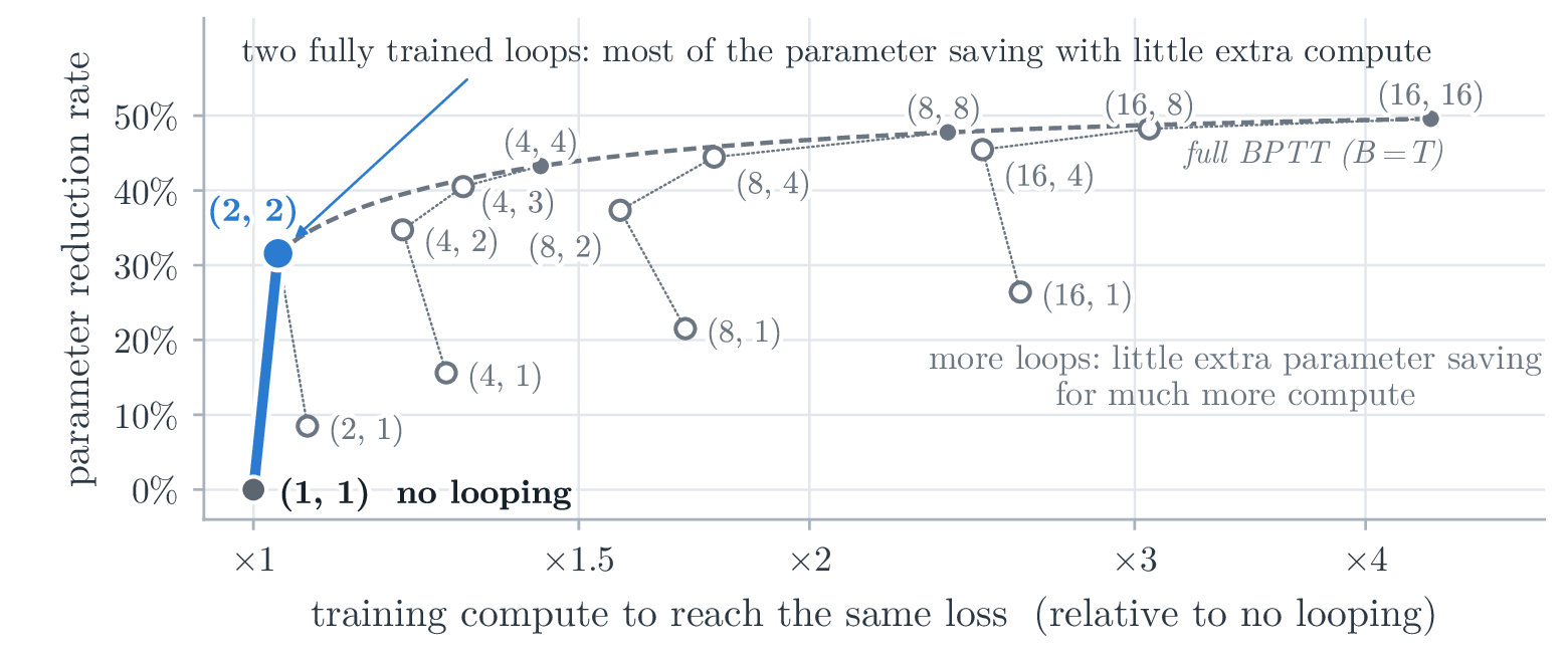
A loop trades compute for parameters: every loop setting needs more compute than the best model without loops, and every one buys a smaller model at the same loss. Every setting has \chi\ge1, so at a fixed compute the best model has no loop, as Schwethelm et al. [4] also find; what a loop offers instead is a discount on parameters, paid for in compute.
Full BPTT forms the frontier: for the same compute, every truncated setting saves fewer parameters, since truncation pays for forward loops that carry no gradient, and its markers lie below the dashed curve of full BPTT.
Two fully trained loops are the knee: (2,2) saves 32% of the parameters for 3.1% more compute, while sixteen loops save 50% of the parameters for 334% more compute. The dense pairs of Section 3.1 measure this knee directly.
| Loop setting | Extra training compute | Parameters saved |
|---|---|---|
| (2, 2) | +3.1% | 31.6% |
| (4, 4) | +43% | 43.3% |
| (8, 8) | +138% | 47.8% |
| (16, 16) | +334% | 49.6% |
Since g\le e^{c}\approx3.04 and half the parameters loop, no setting can save more than 1-1/(0.49+0.51\cdot3.04)\approx51\% of the parameters, whatever the compute (Tab. 6). The first step is cheap because sharing costs little. Replace the shared block of a (2,2) model with two untied copies: the copies cost the same compute per token, but they are worth N_{\text{once}}+2N_{\text{rec}} effective parameters, against N_{\text{once}}+g(2,2)\,N_{\text{rec}} for the shared block. With g(2,2)\approx1.91, sharing loses only 9% of one copy while storing half the recurrent weights; Fig. 6 shows how this gap widens for more loops.
Conclusions
We asked how many parameters a loop saves at the same training compute. In dense models, compute-optimal (2,2) models match the best models without loops with 27–32% fewer parameters at the same training compute, and beat them with 27% fewer parameters for 8% more training compute. In mixture-of-experts models, where the experts hold nearly all of the parameters, sharing the experts across loops saves 17% of the parameters for 9% more compute per token, and sharing every weight saves 11% of the parameters and beats the untied twin for 18% more compute per token.
A scaling law fitted to nearly 600 training runs explains the trade. It prices every loop setting in effective parameters, and read at equal loss it gives a parameter–compute Pareto frontier: no loop is free, full BPTT forms the frontier, and two fully trained loops are its knee, saving about a third of the parameters for 3% more compute.
A loop therefore moves the cost of a model from memory to computation. That trade pays whenever the parameters, rather than the training compute, are the binding budget.