

Looped transformerstruncated BPTTscaling laws

Truncate or Not?

A Scaling Study of Looped Transformers with Truncated Backpropagation

Xuyuan Xiong1,* Siyu Chen2,* Zihan Shao2 Yue Su1 Weiyang Jin1 Ping Luo1 Zhuoran Yang2,† Xihui Liu1,†

1MMLab, The University of Hong Kong 2Yale University

*Equal contribution   †Corresponding authors

HKU MMLab The University of Hong Kong Yale University
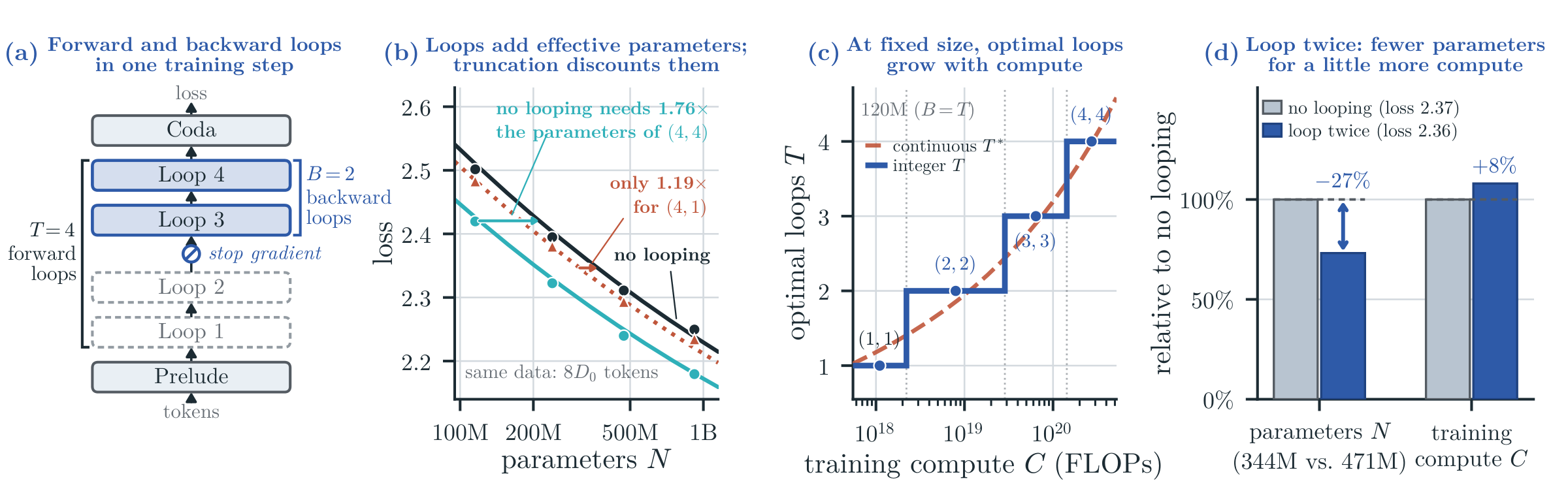
Four-panel overview: a training step with four forward loops of which the last two are trained; loss against parameters for no looping, (4,4) and (4,1); the optimal loop count growing with compute at fixed size; and a two-loop model with 27% fewer parameters beating a non-looped model for 8% more compute.
Overview of looped transformer scaling with truncated BPTT. (a) One training step for \((T,B)=(4,2)\): \(T\) forward loops, of which the last \(B\) are trained. (b) At \(8D_0\) tokens, loops add effective parameters while truncation discounts them (lines: law, markers: runs). (c) At a fixed size (120M), the optimal \(T\) grows with compute under full BPTT. (d) \((2,2)\) at 344M beats \((1,1)\) at 471M and \(2.1\times10^{19}\) FLOPs in loss (2.36 vs. 2.37 nats) with 27% fewer parameters and 8% more compute.
TL;DR

Truncated backpropagation through time (BPTT) trains only the last \(B\) of \(T\) loops of a looped transformer to save compute. We fit one scaling law over model size, data and both loop counts, in which loops add effective parameters and truncation discounts them. Its answer to the title: truncate only when the number of forward loops is fixed in advance. When both loop counts can be chosen, use full BPTT through fewer loops. With model size free as well, the law favors no looping, and two fully trained loops come closest, saving about 30% of the parameters for little extra compute (figure below).

592training runs
58M–919Mnon-embedding parameters
15loop settings \((T,B)\), \(T\le16\)
0.9992\(R^2\) of one law with nine coefficients
Abstract

Looped transformers reuse a shared block of layers to increase computational depth without increasing the number of trainable parameters. They are trained with backpropagation through time (BPTT). To save training compute, BPTT is often truncated to the last few loops, but truncation yields biased gradients that may weaken the benefit of looping. In this work, we study the value of truncation in looped transformer training in a systematic way: we jointly vary model size, training tokens, and forward and backward loop counts across nearly 600 training runs and fit a unified scaling law that captures the effects of looping and truncation through effective parameters. Despite the training-compute savings of truncation, our fitted law favors full BPTT when forward and backward loop counts are jointly optimized. In matched-compute runs, full BPTT through fewer loops consistently outperforms truncated settings of the same compute. The law further shows that at fixed model size, the compute-optimal loop count and training-token budget both grow with compute. When model size is also free, the law identifies two fully trained loops as the best looped setting. Experimentally, this setting achieves lower validation loss than the compute-optimal non-looped model with about 27% fewer non-embedding parameters and only 8% more training compute.

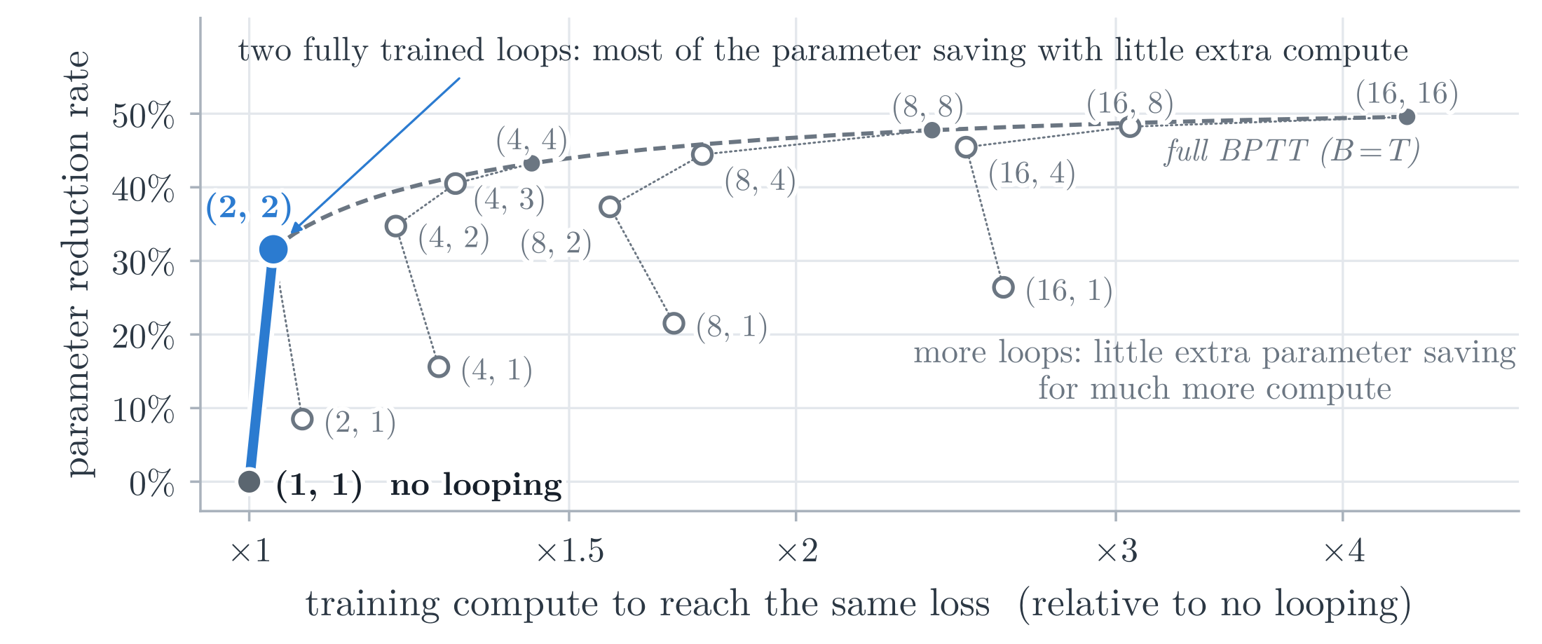
Each loop setting placed by the training compute it needs to match the loss of no looping and the fraction of non-embedding parameters it saves; the fully trained settings form the upper frontier, every truncated setting lies below it, and two fully trained loops save about 30% of the parameters with little extra compute.
No looping is computationally optimal; two fully trained loops save most parameters with little extra compute. Each marker is a loop setting \((T,B)\), with \(T\) forward loops and the last \(B\) trained, at the parameter and token counts our scaling law finds compute-optimal. Compared with the model without looping at the same loss, the horizontal axis shows the training compute it needs and the vertical axis the fraction of non-embedding parameters it saves. Filled markers use full BPTT (\(B=T\)), and the dashed curve is the law's prediction for full BPTT at any \(T\) from 2 to 16. Every truncated setting lies below this curve, so full BPTT forms the frontier and saves the most parameters at each compute.

Four findings

Finding 1

Loops add effective parameters; truncation discounts them

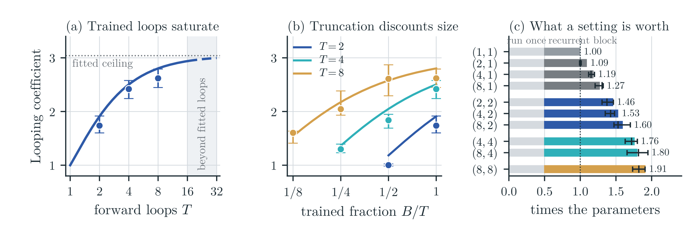
We measure what looping is worth by an effective parameter count: the size of a non-looped model that reaches the same loss on the same tokens. Each fully trained loop adds effective parameters, with diminishing returns toward a finite ceiling. Truncation discounts this gain, and from the same setting, doubling \(B\) adds more effective parameters than doubling \(T\).

  • (4, 4) is worth 1.76× its parameters
  • (4, 1) only 1.19×
Three panels: the looping coefficient with full BPTT saturating toward a ceiling near 3; the coefficient against the trained fraction B over T for T equal to 2, 4 and 8; and the effective size of each loop setting in multiples of the parameters.
What a loop setting is worth in effective size. (a) With full BPTT, the looping coefficient \(g(T,T)\) approaches its fitted ceiling. (b) \(g(T,B)\) against the trained fraction \(B/T\). (c) Total effective size \(N_{\mathrm{eff}}/N\), grouped by \(B\). Lines, bars and numbers: the law; markers: run estimates (median and interquartile range over sizes and budgets). Effective size is set mainly by \(B\): within each group of equal \(B\), neither the law nor the runs gain much from more forward loops.
Finding 2

Truncation helps only at a prescribed forward-loop count; otherwise full BPTT is optimal

A forward pass through the recurrent block costs one unit of compute and a backward pass two, so a loop setting \((T,B)\) costs \(T+2B\) units per token: \((8,2)\) and \((4,4)\) cost the same. Whether truncation pays depends on what is held fixed.

\(T\) prescribed

Truncate

The saved backward compute buys a larger model and more tokens, which more than offset the discounted loop gain. At \(T=8\) the law picks \(B^*=2\); laws fitted separately at \(T=4\) and \(T=8\) agree.

34% less compute at equal loss for \((8,2)\) vs. \((8,8)\)

\(T\) and \(B\) both chosen

Full BPTT

At fixed loop compute, one backward loop is worth more than the two forward loops of the same cost (\(q\approx1.02>2p\approx0.47\)), so the law is maximized with every loop trained. Rather than stopping gradients on early loops, run fewer loops and train them all.

5 / 5 model sizes where \((4,4)\) beats the equal-cost \((8,2)\)

SizeCompute \(C\) (\(10^{19}\) FLOPs)Loss \((8,2)\)Loss \((4,4)\)\(\Delta L\)
60M2.412.52112.49330.0278
120M4.592.38432.36960.0147
240M8.282.27782.26420.0136
480M15.292.18452.17380.0107
1B28.382.11442.10570.0087
Reducing forward depth at equal training compute. Measured validation loss at \(D=16D_0\) (17.2B tokens), in nats per token. Within each row, \((8,2)\) and \((4,4)\) have the same model size, tokens and training compute; \(\Delta L = L_{8,2}-L_{4,4}\).
Finding 3

At fixed model size, optimal loops and tokens both grow with compute; tokens grow faster

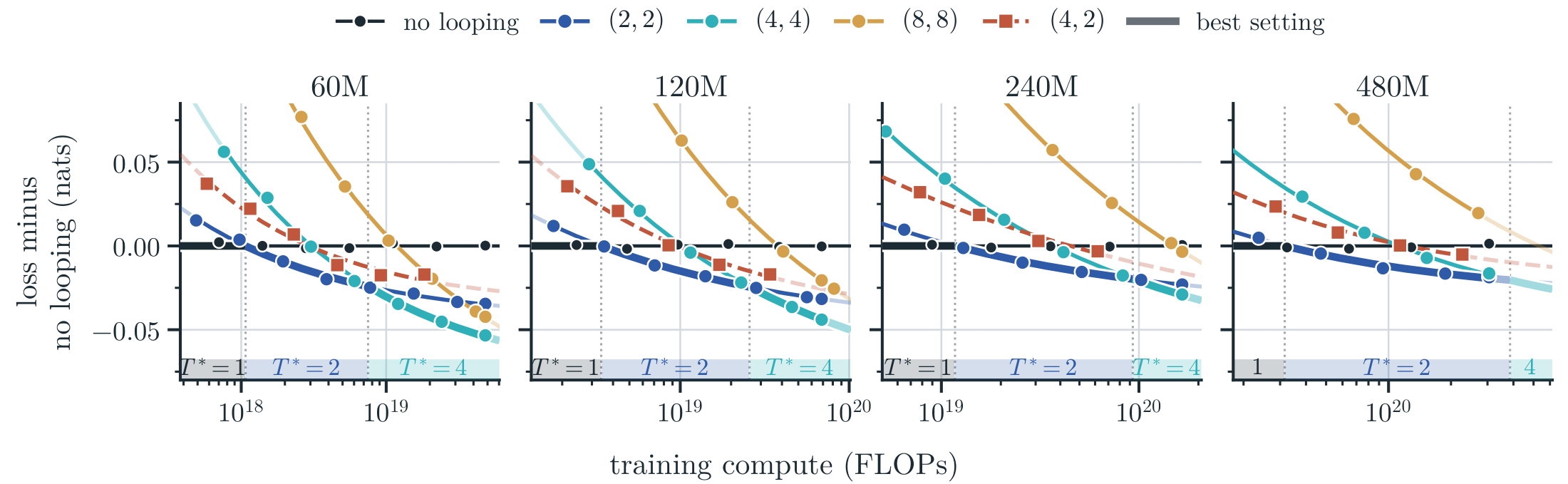
When a model must fit a memory budget, extra compute can buy more loops per token or more training tokens. Under the fitted law with full BPTT, the compute-optimal loop count grows as \(C^{0.24}\) and the token count as \(C^{0.76}\), where \(C\) is the training compute; the runs at every size agree.

Loop counts are integers, so the best setting changes in steps: no looping, then two, then four trained loops. Between steps, added compute goes to tokens.

10× more compute at a fixed size

loops \(T^*\propto C^{0.24}\) ×1.7
tokens \(D^*\propto C^{0.76}\) ×5.8
Loss relative to no looping against training compute at 60M, 120M, 240M and 480M; the best setting switches from no looping to two and then four fully trained loops as compute grows.
At a fixed model size, the best loop count grows with training compute: no looping, then two, then four trained loops. Loss minus that of the model without looping at the same compute, which spends it on more tokens; markers are runs, with a smooth curve through each setting; \((4,2)\) trains half of its four loops. The bold curve is the best setting, named in the strip by its loop count \(T^*\) (faded where extrapolated).
Finding 4

With free model size, no looping is optimal, but two fully trained loops come close with 27–32% fewer parameters

When model size is free, compute spent repeating a block could instead train more unique parameters, so the law favors no looping at every compute (figure above). Among looped settings, \((2,2)\) comes closest: \(g(2,2)\approx1.91\), so two shared loops are worth almost two untied copies of the block.

In the runs, the compute-optimal \((2,2)\) model stays within 0.008 nats of the compute-optimal model without looping at equal training compute, with 27–32% fewer non-embedding parameters. With 8% more compute, its loss falls below.

What is a loop setting worth?

Pick forward loops \(T\) and backward loops \(B\). The numbers come from the fitted law; try a truncated setting such as \((8,2)\) and compare it with full BPTT at the same compute.

8
2
forward only, no gradient trained (backpropagated) stop gradient
This setting (8, 2)
12 units
Full BPTT, same compute
12 units

forward unit   backward unit (2 per trained loop)

Looping coefficient g(T, B) – 1 = no looping, ceiling 3.04
Effective size Neff / N – the parameters of a non-looped model
Training compute per token – relative to no looping
Compute per effective parameter – lower is better
If \(T\) is prescribed

If \(T\) can be chosen too

Fitted coefficients \(c=1.112\), \(p=0.237\), \(q=1.022\); \(N_{\mathrm{rec}}/N=0.507\) as in the 240M model. Compute per token is the leading-FLOP count \(6N_{\mathrm{comp}}\) with \(N_{\mathrm{comp}}=N_{\mathrm{once}}+\tfrac{T+2B}{3}N_{\mathrm{rec}}\); at equal loss, training compute is proportional to compute per effective parameter. Runs cover \(T\le16\).

One law for size, data and loops

The validation loss follows a coupled size–data law in which the model size is replaced by the effective size. The looping coefficient adds three coefficients \(c,p,q\) to the six of the size–data law; all nine are fitted jointly on 230 configurations (\(R^2=0.9992\)).

\[L(N,D,T,B) \;=\; E + \left[A\left(\frac{N_{\mathrm{eff}}}{N_0}\right)^{-\alpha} + H\left(\frac{D}{D_0}\right)^{-\beta}\right]^{\kappa}\] \[N_{\mathrm{eff}} = N_{\mathrm{once}} + g(T,B)\,N_{\mathrm{rec}}, \qquad g(T,B) = \exp\!\big[c\,\big(1 - T^{-p}B^{-q}\big)\big]\]
Normalization \(g(1,1)=1\)

A single loop recovers the non-looped model.

Monotonicity \(\partial_T g>0,\ \partial_B g>0\)

More loops of either kind raise the coefficient.

Zero-backward boundary \(g(T,0)=0\)

An untrained recurrent block adds no effective size.

Saturation \(g\le e^{c}\approx3.04\)

Finite parameters store finite information.

Size–data law

\(E\)\(A\)\(H\)\(\alpha\)\(\beta\)\(\kappa\)
0.29866.48707.63340.30570.39280.3251

Looping coefficient

\(c\)\(p\)\(q\)
1.11200.23681.0218

Reference scales \(N_0=2.4\times10^{8}\) non-embedding parameters and \(D_0=2^{30}\approx1.07\times10^{9}\) tokens; loss in nats per token on deduplicated held-out data.

Citation

@misc{xiong2026truncate,
  title         = {{Truncate or Not? A Scaling Study of Looped Transformers
                    with Truncated Backpropagation}},
  author        = {Xuyuan Xiong and Siyu Chen and Zihan Shao and Yue Su and
                   Weiyang Jin and Ping Luo and Zhuoran Yang and Xihui Liu},
  year          = {2026},
  eprint        = {2610.26030},
  archivePrefix = {arXiv},
  primaryClass  = {cs.LG},
  url           = {https://arxiv.org/abs/2610.26030}
}

Acknowledgements

This work builds on the looped language model architecture, data pipeline, and MuonH + HyperP training recipe of Schwethelm et al. (2026) (kschwethelm/looped-lm-scaling) and on the recurrent-depth design of Huginn (Geiping et al., 2025). We thank the authors for releasing their code.